The Buzz on Vlookup Excel
array _ lookup: It is defined whether you want an exact or an approximate suit. The feasible value holds true or FALSE. Real value returns an approximate suit, and also the FALSE worth returns a specific match. The IFERROR function returns a value one defines id a formula assesses to an error, or else, returns the formula.
IFERROR look for the list below mistakes: #N/ A, #VALUE!, #REF!, #DIV/ 0!, #NUM!, #NAME?, or #NULL! Keep in mind: If lookup _ worth to be browsed happens greater than once, then the VLOOKUP feature will certainly locate the initial event of lookup _ worth. Below is the IFERROR Formula in Excel: The arguments of IFERROR function are discussed listed below: worth: It is the worth, recommendation, or formula to look for an error.
While making use of the VLOOKUP function in MS Excel, if the value looked for is not discovered in the provided information, it returns #N/ A mistake. Below is the IFERROR with VLOOKUP Solution in Excel: =IFERROR( VLOOKUP (lookup _ worth, table _ variety, col _ index _ num, [range _ lookup], worth _ if _ error) IFERROR with VLOOKUP in Excel is very straightforward and also easy to make use of.
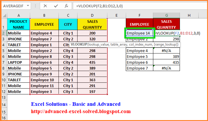
You can download this IFERROR with VLOOKUP Excel Design Template below-- IFERROR with VLOOKUP Excel Theme Allow us take an example of the standard pay of the staff members of a business. In the above figure, we have a checklist of employee ID, Staff member Call as well as Worker standard pay. Currently, we intend to look the workers 'basic pay with respect to the Worker ID 5902. In this scenario, VLOOKUP function will return #N/ An error. So it is better to replace the #N/ An error with a personalized value that everyone can comprehend why the mistake is coming. So, we will certainly utilize IFERROR with VLOOKUP Feature in Master the list below way:=IFERROR (VLOOKUP (F 5, B 3:D 13, 3,0)," Data Not Found" )We will certainly observe that the mistake has actually been changed with the tailored value "Information Not Found". We can make use of the function in the exact same workbook or from various workbooks by the use 3D


cell referencing. Let us take the instance on the same worksheet to recognize the use of the feature on the fragmented datasets in the very same worksheet. In the above number, we have two sets of information of basic pay of the staff members. Currently, we intend to look the staff members' standard pay relative to the Employee ID
Not known Factual Statements About How To Use Vlookup
5902. We will utilize the following formula for browsing data in table 1:=VLOOKUP (G 18, C 6: E 16, 3, 0)The outcome will come as #N/ A. As the information browsed for is not available in the table 1 information set. The employee ID 5902 is readily available in Table 2 information set. Currently, we desire to contrast both of the information sets
of table 1 and table 2 in a solitary cell and get the outcome. It is much better to change the #N/ A mistake with a customized worth that everybody can recognize why the error is coming. So, we will certainly use IFERROR with VLOOKUP Feature in Excel in the list below means:=IFERROR(VLOOKUP(lookup _ worth, table _ array, col _ index _ num, [array _ lookup], IFERROR (VLOOKUP (lookup _ worth, table _ array, col _ index _ num, [range _ lookup], worth _ if _ mistake)) We have used the function in the instance in the list below method: =IFERROR(VLOOKUP(G 18, C 6: E 16, 3,0), IFERROR (VLOOKUP (G 18, J 6: L 16, 3, 0),"Data Not Found"))As the staff member ID 5902 is readily available in the table 2 information established, the result will reveal as 9310. Pros: Useful to trap as well as manage mistakes created by various other solutions or features. IFERROR checks for the following mistakes: #N/ A, #VALUE!, #REF!, #DIV/ 0!, #NUM!, #NAME?, or #NULL! Cons: IFERROR replaces all kinds of mistakes with the tailored worth. If any type of other errors except the #N/ An occur, still the tailored value defined will be viewed in the outcome. If value _ if _ mistake is provided as a vacant message(""), nothing is shown also when an error is discovered. If IFERROR is offered as a table variety formula, it returns a selection of outcomes with one thing per cell in the worth field. This has actually been a guide to IFERROR with VLOOKUP in Excel. You can additionally govia our other suggested short articles-- How to Make Use Of RANKING Excel Function Function HLOOKUP Function in Excel With Examples Exactly How To Make Use Of ISERROR Feature in Excel. VLOOKUP is an extremely helpful formula in Excel. Sadly -- for the SEM novice-- it is additionally one of the most complex when you are just beginning. Given that I 'm a relative beginner in paid search, the brunt of my work is production jobs. VLOOKUP is something that I use every day. Obviously I requested for aid, yet discovering VLOOKUP from someone who currently understood it and its complexities confirmed to be not so helpful. I frantically wanted somebody to simply lay it out in the plainest, most stripped-down way feasible. To ensure that's what I will certainly do for you below: I'll walk you with the framework actions that I want I had actually understood. I don't also know every little thing it can do yet. )According to Excel's formula description, VLOOKUP"tries to find a worth in the leftmost column of a table, and afterwards returns a value in the exact same row from a column you specify. "Super practical, appropriate? To stupid it down for you
, VLOOKUP lets you draw details about your picked cells into your existing sheet, from various other sheets or workbooks where that value exists. CPC for each and every keyword is. You have another sheet that is a keyword record with all the data for every single keyword phrase in the account-- this will be called Key words Sheet. You can avoid by hand sorting with every one of those key words and needing to duplicate and paste the Avg. CPCs by utilizing VLOOKUP.
excel vlookup in marathi vlookup in excel using python vlookup in excel uipath